Annotated R code to create the maps and results in my post “15 minutes from the Lee-to-Sea Greenway“.
My route was calculated by Google maps using a small number of waypoints to generate a cycle route plan and should be displayed on https://www.google.com/maps/dir/51.9047276,-8.6610302/Passage+West/51.7976563,-8.2762756/@51.8633137,-8.5142921,11z/data=!4m10!4m9!1m0!1m5!1m1!1s0x4844849b81c2dae5:0xa00c7a99731cef0!2m2!1d-8.3362128!2d51.8720626!1m0!3e1 (although I imagine this might be recalculated differently at different times, if new data or traffic levels redirect the algorithm).
A calculated Google Maps route can be converted to a GPX file in many ways, including pasting the route link (above) into the online converter at https://mapstogpx.com/
Preliminaries
Having installed the language R and some kind of environment, such as R Studio, install the packages rgdal, rgeos and (if you want to convert text addresses to locations) tidygeocoder. The following code loads the necessary packages and defines a function to generate semi-transparent colours, to add coloured overlays to maps.
# Load package libraries
library(rgdal)
library(rgeos)

# Add transparency to standard colour definitions
add.alpha <- function(COLORS, ALPHA=0.5){
  RGB <- col2rgb(COLORS, alpha=TRUE)
  RGB[4,] <- round(RGB[4,]*ALPHA)
  NEW.COLORS <- rgb(RGB[1,], RGB[2,], RGB[3,], RGB[4,], maxColorValue = 255)
  return(NEW.COLORS)
}
The Small Area Populaton Statistics (SAPS) aggregate the 2016 census by Electoral Division and areavailable in a variety of formats from the CSO SAPS website 2016. The CSV file contains a comma thousands separator in numbers, which can be read as follows:
setClass("num.with.commas")
setAs("character", "num.with.commas", function(from) as.numeric(gsub(",", "", from)))
d2016 <- read.csv("SAPS 2016/SAPS2016_ED3409.csv",colClasses = c("character", "character", "character", rep("num.with.commas",798)))
If you have a SAPS shapefile, it will already contain mapping data (polygons), but if not then merge the SAPS data with the ED boundary shapefile, available from the CSO. It will be necessary to make the ED IDs match by adding “ED2409_” to the shapefile, or deleting it from the SAPS dataframe.
ed <- readOGR("electoral_divisions.shp", encoding = "ISO8859-1")
ed$CSOED <- paste("ED3409_", ed$CSOED, sep="")
ed@data <- merge(ed@data, d2016, by.x = c("CSOED"), by.y = c("GEOGID"), all.x=TRUE, sort=FALSE)
The combined ED shapefile and SAPS data cover the whole country. Limit the data to Cork City and Cork County, in a new shape “temp”. For ease of reading the map later on, I have sorted the EDs by West and then North, so any table will read from left to right across the map:
# Limit the data to just the counties of interest
county <- c("Cork City", "Cork County")
temp <- ed[ed$COUNTYNAME%in%county,]
# Find the centroid of each ED
temp@data$x <- gCentroid(temp,byid=TRUE)$x
temp@data$y <- gCentroid(temp,byid=TRUE)$y
temp <- temp[order(temp$x,temp$y),]
plot(temp, col="lightgreen", border="darkgreen", bg="blue")
Read route from GPX file (extracted from Google Maps) and transform the coordinates to the same map projection as the ED shapefile. Then add a buffer (a radius, extended over the whole route) of 2 km and 6 km, to create a route, route2km which is a 4 km thick line and route6km which is a 6 km thick line. Exclude the EDs North of the Lee and far from bridges:
route <- readOGR("mapstogpx20210206_173113.gpx",layer="tracks")
route <- spTransform(route,temp@proj4string)
route2km <- gBuffer(route,width=2000)
route2km <- gIntersection(route2km, temp[!temp$EDNAME%in%c("Caherlag", "Carrigtohill", "Cobh Rural", "Cobh Urban", "Corkbeg", "Inch", "Rathcooney", "Riverstown"),])
route6km <- gBuffer(route,width=6000)
route6km <- gIntersection(route6km, temp[!temp$EDNAME%in%c("Caherlag", "Carrigtohill", "Cobh Rural", "Cobh Urban", "Corkbeg", "Inch", "Rathcooney", "Riverstown"),])
Add new fields r (the route passes inside ED), r2km (the route passes within 2km) and r6km (the route passes within 6km). Reduce the temp shape even further to only those EDs on the route, in a new variable “temp.route”.
# EDs through which the route passes
temp@data$r <- as.vector(gCrosses(temp,route,byid=TRUE))
temp@data[temp$r==TRUE, c("OSIED","EDNAME")]
# EDs with land within the 2km buffer
temp@data$r2km <- as.vector(gIntersects(temp,route2km,byid=TRUE))
temp@data[temp$r2km==TRUE, c("OSIED","EDNAME", "r", "r2km")]
# EDs with land within the 6 km buffer
temp@data$r6km <- as.vector(gIntersects(temp,route6km,byid=TRUE))
temp@data[temp$r6km==TRUE, c("OSIED","EDNAME", "r", "r2km", "r6km")]
# New variable of just the EDs of interest
temp.route <- temp[temp$r6km,]
Estimate population within 2 km and 6 km (assuming even population density), simply by measuring the area intersecting the buffer as a proportion of total area. Save these area proportions, and save the estimated proportion of population. Write the result as a CSV spreadsheet file:
temp.route@data$p2km <- 0
temp.route@data$p6km <- 0
for (i in 1:length(temp.route)){
  common <- gIntersection(temp.route[i,],route2km)
  if (!is.null(common)) {
    temp.route@data$p2km[i] <- gArea(common) / gArea(temp.route[i,])
  }
  common <- gIntersection(temp.route[i,],route6km)
  if (!is.null(common)) {
    temp.route@data$p6km[i] <- gArea(common) / gArea(temp.route[i,])
  }
}
temp.route@data$pop2km <- as.integer(temp.route@data$T1_1AGETT * temp.route@data$p2km)
temp.route@data$pop6km <- as.integer(temp.route@data$T1_1AGETT * temp.route@data$p6km)
# Total population within 2 km and 6 km, output table
sum(temp.route$pop2km)
sum(temp.route$pop6km)
write.csv(temp.route@data[, c("OSIED","EDNAME", "T1_1AGETT", "r", "r2km", "p2km", "pop2km", "r6km", "p6km", "pop6km")], "Lee to Sea.csv")
Corinne landcover data, from the EPA, provides an attractive base map useful visual information about the route of the greenway, distinguishing woods, vegetation, urban space, inland marshes, water bodies and sea. I have used brown, green, light green, yellow and blue to create a vegetation, built, tidal and water distinction. We only need a small portion, and using the bounding box of temp.route to define the plot area, then plot the Corinne map falling within this bounding box as a base layer for the route map. The Corinne map has to be transformed, as with the route GPX data, to the same map projection as the ED shapefile.:
corinne <- readOGR("Maps of Ireland/CLC18_IE_ITM/CLC18_IE_ITM.shp")
corinne <- spTransform(corinne,temp@proj4string)
corinne.colours <- c("Continuous urban fabric"="brown", "Discontinuous urban fabric"="brown", "Industrial or commercial units"="brown", "Road and rail networks and associated land"="brown", "Port areas"="brown", "Airports"="brown", "Mineral extraction sites"="brown", "Dump sites"="brown", "Construction sites"="brown", "Green urban areas"="green", "Sport and leisure facilities"="green", "Non-irrigated arable land"="green", "Fruit trees and berry plantations"="green", "Pastures"="green", "Complex cultivation patterns"="green", "Land principally occupied by agriculture, with significant areas of natural vegetation"="green", "Broad-leaved forest"="green", "Coniferous forest"="green", "Mixed forest"="green", "Natural grasslands"="green", "Moors and heathland"="green", "Transitional woodland-shrub"="green", "Beaches, dunes, sands"="yellow", "Bare rocks"="yellow", "Sparsely vegetated areas"="yellow", "Burnt areas"="yellow", "Inland marshes"="lightgreen", "Peat bogs"="lightgreen", "Salt marshes"="lightgreen", "Intertidal flats"="lightgreen", "Water courses"="blue", "Water bodies"="blue", "Coastal lagoons"="blue", "Estuaries"="blue", "Sea and ocean"="blue")
Route map
The Lee to Sea route map is plotted by first plotting a blue (sea) bounding box to contain the entire route. The map is then plotted as a Corinne land use underlay, the ED boundaries of Cork (from temp), the emphasised EDs adjacent to the route (from temp.route), with text labels for large EDs, and finally the 6 km and 2 km buffers and route.
png("Lea to sea.png",width=2000,height=1500)
# Plot a bounding box
plot(bbox2SP(bbox=bbox(temp.route)),bg="blue",border=NA)
# Aesthetic map of land use
plot(corinne, add=TRUE, col=corinne.colours[corinne@data$Class_Desc])
plot(temp.route, add=TRUE,col=add.alpha("lightgray",0.1), border="darkgreen", bg="lightblue")
# Outlying EDs
plot(temp, add=TRUE, col="transparent",border="gray")
# EDs on the route, with labels if they are large enough
plot(temp.route, add=TRUE, col=add.alpha("white",0.2), border="black")
text(coordinates(temp.route),labels=temp.route$EDNAME,col=ifelse(temp.route@data$TOTAL_AREA>10,"black","transparent"))
# Plot the 6 km and 2 km buffers, and the route in 8 px red
plot(route6km, add=TRUE, col=add.alpha("red", 0.2), border=add.alpha("red",0.6))
plot(route2km, add=TRUE, col=add.alpha("red", 0.2), border=add.alpha("red",0.6))
plot(route, add=TRUE, col="red", lwd=8)
dev.off()
Schools Map
A complete list of post-primary schools (and national schools) is available from the Department for Education. The official name and address are sufficient to automatically geocode about 60% of schools using the freely accessible Open Street Maps Nominatum service, or 100% using a subscription Google Maps lookup. Assuming you have already added longitude and latitude to the schools (see below), the following code will plot the schools over a simplified route map. You could add school labels.
secondary <- read.csv("post-primary-schools-location-2019-2020.csv")
png("Lea to Sea - schools.png",width=2000,height=1500)
# Plot a bounding box around the route
plot(bbox2SP(bbox=bbox(temp.route)),bg="blue",border=NA)
# Add all ED boundaries and highlight those adjacent to the route
plot(temp,add=TRUE,col="lightgray",border="black")
plot(temp.route, add=TRUE,col=add.alpha("lightgray",0.1), border="darkgreen", bg="lightblue")
plot(temp, add=TRUE, col="transparent",border="gray")
plot(temp.route, add=TRUE, col=add.alpha("white",0.2), border="black")
text(coordinates(temp.route),labels=temp.route$EDNAME,col=ifelse(temp.route@data$TOTAL_AREA>10,"black","transparent"))
# Plot the 2 km and 6 km buffers and route
plot(route6km, add=TRUE, col=add.alpha("red", 0.2), border=add.alpha("red",0.6))
plot(route2km, add=TRUE, col=add.alpha("red", 0.2), border=add.alpha("red",0.6))
plot(route, add=TRUE, col="red", lwd=8)

# Calculate which zone, 0=none, 2=2km or 6=6km schools lies in
secondary$zone <- 0
for (i in 1:nrow(secondary)){
  # For each school in Cork County
  if (secondary$County[i]=="Cork"){
    # Convert the latitude and longitude to a spatial point
    lat<-as.numeric(secondary$latitude[i])
    long<-as.numeric(secondary$longitude[i])
    coords<-cbind(long, lat)
    sp <- SpatialPoints(coords, proj4string=CRS("+proj=longlat +datum=WGS84 +no_defs"))
    # Transform to the same map projection as the ED shapefile
    sp <- spTransform(sp,temp@proj4string)
    # Plot a black X outside the route, white or green dot inside
    col<-"black" ; pch<-4
    if(gIntersects(sp,route6km)) {
      col<-"green" ; pch<-20 ; secondary$zone[i]<-6
    }
    if(gIntersects(sp,route2km)) {
      col<-"white" ; pch=20 ; secondary$zone[i]<-2
    }
    points(spTransform(sp,temp@proj4string), pch=pch, col=col, cex=2)
  }
}
dev.off()

# List schools within 2 km, number of schools, total of pupils
secondary[secondary$zone==2,c("Official.School.Name","TOTAL..2019.20.")]
nrow(secondary[secondary$zone==2,])
sum(secondary[secondary$zone==2,"TOTAL..2019.20."])

# List schools within 6 km, number of schools, total of pupils
secondary[secondary$zone==6,c("Official.School.Name","TOTAL..2019.20.")]
nrow(secondary[secondary$zone==6,])
sum(secondary[secondary$zone==6,"TOTAL..2019.20."])
nrow(secondary[secondary$County=="Cork",])
plot(temp[temp$EDNAME=="Douglas",],col=add.alpha("purple",0.1), add=TRUE)
School Locations
If you have a Google Maps API subscription, then follow instructions using ggplot and ggmap, which will have a far higher success rate (and should be 100% complete with Eircodes). I used the freely accessible Open Street Maps for an initial pass through the school addresses, adding about 60% of locations autoimatically. I then listed the Eircodes of schools with no location (in Cork only) and manually added the longitude and latitude from a (manual) Google Maps search.
library(tidygeocoder)
# Test the geocoder
geo(address="44 MacCurtain Street, Cork, Ireland",method="osm")

# Read the post-primary file, adding empty location fields
secondary <- read.csv("~/Downloads/post-primary-schools-2019-2020.csv")
secondary$latitude <- NA
secondary$longitude <- NA

# Combine the non-blank address lines, adding "Ireland"
secondary$address <- paste(secondary$Official.School.Name,
ifelse(secondary$Address.1!="",paste(", ",secondary$Address.1,sep=""),""),
ifelse(secondary$Address.2!="",paste(", ",secondary$Address.2,sep=""),""),
ifelse(secondary$Address.3!="",paste(", ",secondary$Address.3,sep=""),""),
ifelse(secondary$Address.4!="",paste(", ",secondary$Address.4,sep=""),""),
", Ireland",sep="")

# Attempt to add geocodes using OSM lookup
for (i in 1:nrow(secondary)){
  if (is.na(secondary$latitude[i])) {
    print(paste(i,"looking up"))
    x <- geo(address=secondary$address[i],method="osm")
    secondary$latitude[i] <- x$lat
    secondary$longitude[i] <- x$long
  }
  else print(paste(i,"done"))
}
# Schools in Cork with no location (for manual search)
# Save in a new file and add latitude and longitude for second pass
secondary[is.na(secondary$latitude)&secondary$County=="Cork","Eircode"]

# Second pass - manual locations from Eircode
eircode <- read.csv("Eircode locations.csv",comment.char="#")
for (i in 1:nrow(secondary)){
  if (is.na(secondary$latitude[i])) {
    print(paste(i,"looking up"))
    x <- eircode[eircode$Eircode==secondary$Eircode[i],]
    if (nrow(x)==1) {
      secondary$latitude[i] <- x$latitude
      secondary$longitude[i] <- x$longitude
    }
  }
  else print(paste(i,"done"))
}

write.csv(secondary, "post-primary-schools-location-2019-2020.csv")
The 15-minute lifestyle
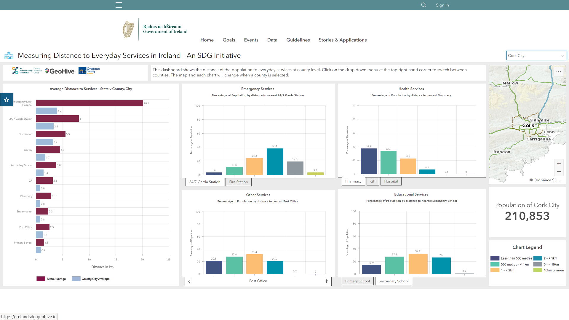
An interesting look at sustainable living is presented in “Measuring Distance to Everyday Services in Ireland – An SDG Initiative” with barcharts of the proportion of population within 500 m, 2km, 5km, 10 km and further than 10 km of everyday services.
The Sustainable Development interactive portal generates barplots of Emergency Services (Garda, Fire Station, Health (Pharmacy, GP and Hospital), everyday services (Post Office, Bank, Supermarket, Swimming Pool, Sports facility) and schools. Plots can be national, county or city based.
One thought on “Annotated analysis of the Lee to Sea data”
Comments are closed.